What Is EPM? Evaluating the Health and Status of Products and Threads (Part 2)

1. BACKGROUND

This paper is the second in a sequence defining Evaluated Product Maturity (EPM).  EPM is designed to assist in assessing the risk of breaking or diminishing the functionality of a system-of-systems functional thread by modifying, changing, or replacing one or more systems that make up that thread.  The sequence of paper provides the basis for computing EPM using BTI’s automated systems and software data science capabilities.

This first document defined the purpose, background, and general approach for computing the EPM score.  

The second installment, which you are currently reading, defines the factors that the data collected from a wide array of systems has indicated is critical in evaluating the risk for changes to a system to break or diminish the functionality of that system.

Future installments will provide the details of calculations, how EPM is automatically calculated from the system of system’s development and maintenance environment, and how information is reported on a near-real-time dashboard.

4. General Approach

4.1 Product Profile

4.1.1 Product Categories/Factors

The following is a list of major groups of categorizations, or factors use in categorizing a system. These factors are then used to calculate the Product Type.

Project Size. Project team size influences both the quality and availability of products as larger teams require more management, oversight and direction, and as size grows so do the communication paths within the group. Increased staff turnover negatively impacts team cohesion; additional mentoring and training become necessary aspects of the team’s development program. 

• Small – 1 to 5 full-time equivalent (FTE) staff
• Medium – 6 to 15 FTEs
• Large – 16 to 50 FTEs
• Very Large – greater than 50 FTEs

Product Group. Products that are stand alone and/or are not part of a larger capability (system, system-of-systems, threads, etc.) are generally less risky and easier to develop and sustain.

• Single Product
• Thread (multiple products and/or cross-product development)

Team Experience (average). Elements considered in this evaluation include programming language experience, application domain experience, familiarity with the toolset, project manager experience and skills.

• Low – less than 2 years
• Medium – 2 to 5 years
• High – greater than 5 years

Application User Base (Size in Users). Products that have a large user base are more difficult to maintain, as both the development and repair cycles may be longer and more resource constrained due to the usual larger numbers of feature requests and bug fixes. 

• Small – 1 to 50 users
• Medium – 51 to 200 users
• Large – greater than 200 users

Process Maturity. Higher maturity positively impacts both development quality and increased productivity.

• Stage 1 – Minimal project management; little or no process definition
• Stage 2 – Overall project management by the numbers; defined processes
• Stage 3 – Processes measured, with continuous improvement
• Stage 4 – Processes optimized, with consistent, excellent performance 

Technical Uncertainty. Uncertainty in the product development process and toolset can lead to unpredictable results in the final product both in terms of quality and deployment frequency. 

• Low – Well known, mature technology
• Medium – Adaption of familiar technology; limited new technology
• High – First use of new technology, previously developed
• Super High – Development of new technology

Critical Application (as determined by Reliability Class)

• Class 0 – 1 not critical to the organization or its customers
• Class 2 – 5 critical to the organization or its customers (2 lowest to 5 highest)

4.12 Product Characterization

Products are characterized into one of four classes, each representing increasing importance, criticality to organization’s goals, risk, etc.  

•  Type-I products are minimal to low risk projects, typically small in size, etc. (for example, an internal text messaging app)
•  Type-II products are low to moderate risk products, moderate in size, etc. (for example, billing software)
•  Type-III products are high risk, large in size, etc. (for example, user authentication)
•  Type-IV products are considered to be of very high risk as multiple factors are valued at the high ends of the scale.

Note that small products with minimal process maturity and high technical uncertainty can be classified higher than large products, with high process maturity and low technical uncertainty. Although there is a relationship between product size and classification, multiple factors are considered in the classification rating as well as differing levels of importance (weights).

The algorithm for classifying a product includes three areas of evaluation. First, each product is scored against a complexity evaluation based on five factors: Product Group, Team Experience, Application User Base, Process Maturity and Technical Uncertainty (see Table 2). Then, product size and whether or not the product is critical are then used to complete the final classification. Each factor has an associated weighting parameter indicating the level of importance of the given factor toward the final evaluation. These weights are fixed for purposes of determining the classification value (See Table 3).

Table 2 – Complexity Factor Enumeration Values

Table 3 – Weighing Factors

The classification value is calculated using the following algorithm:

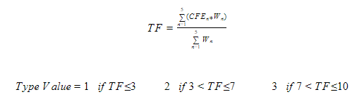
Type Value is increased by 1 if the following conditions are met:

• The Product Size is Small to Medium and TF > 7
• The Product Size is Large and TF >= 3
• The Product Size is Very Large

Critical products cannot be classified lower than Type Value 3. Therefore mission critical products, those with an assigned reliability class of Class-2 to Class-3, which are evaluated as Type Value 1 or 2 are automatically upgraded to Type Value 3. Those with reliability classes of Class-4 or Class-5 are upgraded to Type Value 4. 

The Product Type identifier is then created as follows:

• Type Value = 1,2,3,4 ? Type-I, Type-II, Type-III, Type-IV
• Mission critical product ? append ‘a’ (e.g. Type-IIa)

4.2 Quantitative Goals

Although products can have any number of specific quantitative goals (some tied to their Product Values) two measures are needed for the model to correctly analyze the EPM value. These measures are the Product’s targeted deployment frequency and change lead time, both used as criteria in measuring the MSI of each metric.

4.3 Selection of Metrics

Measures and metrics are categorized into five groups (not necessarily mutually exclusive) and are used in the evaluation/monitoring of a product. 

• Performance
• Support (QA and CM)
• Software Vulnerabilities
• Management
• Service

Some measures are required (see Table 4); others are based on value statements and key goals of the product management and customer needs and would typically be used for the extended evaluations. Selection is based on the Product Profile (note that not all product types need all metrics – Help Desks, for example, need only Service and Management metrics).

Because of the type of processes (and specific measures collected) for service based products, implicit maturity evaluations of these products cannot be used in comparisons to non-service based products. A separate health and status (and maturity) evaluation needs to be developed to address these types of products. 

4.4 Assigning Thresholds

The next measure of product EPM is determined through an evaluation of measurement thresholds that are derived from the performance, quality and software vulnerabilities objectives of a product. This evaluation determines the MSI for each metric. In the case of the extended evaluations these are based on product “value statements”, which are customer/user based statements of key/critical aspects of product capability and are selected based on organization leadership goals. 

Threshold numbers are typically given in terms of a maximum (or minimum) values, and may include ranges to provide the degree of allowable acceptance. For example, a product may establish the following thresholds:

Mean Code Complexity per file

• >= 50 ? Red
• >= 20 ? Yellow
• < 20 ? Green

Compliance Code Test Coverage

• < 95% ? Red
• otherwise ? Green

Some metrics (DF, CLT, TTR, NTR and AUC) are evaluated based on their mean values over time and therefore do not contribute to EPM scores until sufficient data is captured for determining a mean value (typically after 4 releases of the product).

Thresholds for the required metrics are pre-determined based on product category as contained in the product profile and are described in the following sections. This standardization is necessary to allow for maturity comparisons among products. Products are free, of course, to establish more or less rigorous thresholds for their own purposes and are encouraged to do so.

Table 4 – Fundamental Metrics

4.4.1 Deployment Frequency (DF)

Rationale: Deployment Frequency (DF) values provide direct and indirect measures of response time, team cohesiveness, developer capabilities and development tool effectiveness. These measures are also required to evaluate whether or not product release schedules are optimized and if teams have the necessary knowledge and resources to complete new capabilities on schedule.

In the traditional life cycle model of development DFs can vary significantly and are usually planned to occur at some specific time as identified in the project schedule. Within an agile development environment, the goal would be deployment frequencies approaching the monthly, weekly, daily levels, and even faster – faster is always better. But when developing in an environment where scheduled sprints are the norm, deployments will typically be “on the sprint cycle”. In these case thresholds for DF are keyed to fixed cycles, and can be evaluated much the same way as in the traditional sense.

For the purpose of monitoring the performance status of a product, the mean deployment frequency (MDF) is evaluated against specified thresholds.

Table 5 – Deployment Frequency Thresholds

4.4.2 Change Lead Time (CLT)

Rationale: The Change Lead Time (CLT) measure provides insight into the efficiency of the development process; the complexity of the code and development systems. This measure is necessary to evaluate the agility of the development team; whether the development process and/or tools are adequate for the task.

Change lead times should strive to be as short as reasonably possible. In many, if not most cases this will be commensurate with the DF, but can be a multiple of the DF as some changes may require more than one sprint to complete. In the traditional environments, CLTs should also be compared against scheduled releases, with values decreasing over time.

For the purpose of monitoring the performance status of a product, the mean change lead time (MCLT) is evaluated against specified thresholds. 

Table 6 – Change Lead Time Thresholds

4.4.3 Time to Repair (TTR)

Rationale: The Time to Repair (TTR) metric is a measure of team effectiveness and capability to respond to issues during the lifetime of the product. It also provides insight into the complexity of the code. Capturing and evaluating this metric is necessary to determine the agility and responsiveness of the product team in repairing defects in the product.

Critical systems need to be highly reliable and as such their TTR should be small. Thresholds for TTR are therefore different for differing product classes. In addition, the severity of the failure needs to be evaluated in concert with the product Type. For example, consider the case where 3 new features are released and one of those fails in the field, but is a minor change to the overall functionality of the product versus a situation where the same single failure is part of a critical change and is absolutely necessary for the product to function correctly. Roll-back, or remedial release in the latter case should occur in a much shorter time frame than in the former case where the user base can deal with the minor inconvenience or have work arounds for the product to remain useful. In the cases when failure severity is critical increase the product Type by one level (with Type-IV being the upper limit) prior to evaluating the status.

For the purpose of monitoring the performance status of a product, the mean time to repair (MTTR) is evaluated against the specified thresholds.

Table 7 – Mean Time to Repair Thresholds

4.4.4 Test Coverage (TC)

Rationale: Test Coverage (TC) measures the overall percentage of code that has been tested via unit tests, and has a direct relationship to the reliability and security of the product. Ideally, all code should be tested. These thresholds provide a sense of reasonableness based on the product Type.

Table 8 – Test Coverage Thresholds

4.4.5 Code Complexity (Comp)

Rationale: Code Complexity is a metric used to indicate the complexity of a program. It is a quantitative measure of the number of linearly independent paths through a program’s source code. In other words, it indicates the number of software tests needed to fully test the code as each path would need to have an associated test. Comp is measured in terms of average code complexity per file. Its importance lies in the fact that more complex code requires more effort to build, test and maintain.

Table 9 – Average Code Complexity Thresholds

4.4.6 Defect Density (DD)

Rationale: Bugs, or defects, are measures of the quality of the product’s code and are directly related to its reliability. Bugs are categorized as Critical, Moderate and Trivial, based on the impact on the functioning of the product. The Defect Density is calculated as the number of bugs per 1,000 lines of code (KLOC). Lower defect density generally implies higher quality in the product. Although there is no industry standard value for defect density (there are too many variables to consider, from the language type to the maturity of the team, to the complexity of the design), values that fall between 1 and 10 defects per KLOC seem to be reasonable expectations for acceptable defect densities.  

Table 10 – Defect Density per severity level

4.4.7 Vulnerability Density (VD)

Rationale: The count of vulnerabilities (vulnerabilities or flaws in programs that can lead to use of the application in a different way than it was designed for) is a measure that groups everything that has to do with design flaws or implementation bugs that can be exploited into a single metric. Security vulnerabilities such as SQL injection or cross-site scripting can result from poor coding and architectural practices. The VD metric thus provides insight into the security of the system code; the higher the value the higher the probability of product failure. Also provides insight into the availability of a product to meet customer needs. The VD is calculated as the number of vulnerabilities per KLOC.

Table 11 – Vulnerability Density per severity level

4.4.8 Code Smell Density (CSD)

Rationale: Code smells are characteristics of the source code that possibly indicate a deeper problem. This is commonly referred to as technical debt – and is directly related to the degree to which the code may exhibit security flaws and maintenance issues. 

By nature, software is expected to change over time, which means that code written today will be updated tomorrow. The ability, cost and time to make such changes in a code base correlates directly to its level of maintainability. In other words, low maintainability means low velocity for development teams. The CSD metric is calculated as the number of code smells per KLOC.

Table 12 – Code Smell Density per severity level

4.4.9 Code Change Rate (CCR)

Rationale: Code Change Rate (CCR) is an indication of the rate at which the code changes over deployments and the degree to which this rate is consistent with the new requirements levied on the product. Abnormally high rates could be a sign of security issues. 

CCR is measured as the amount of code changes per deployment (ratio of the number of changed/new LOC to total new requirements/bug fixes). Because of the nature of the underlying dependencies (code complexity, type of change, code language, etc.), this metric needs to be evaluated in terms of a consistent or gradually decreasing value over time. Products need to identify their own value for the average number of LOC required per requirement/bug fix and use that in the evaluation of CCR. For example, a code change that produces a change in CCR that is over three times the standard deviation of the Mean CCR would indicate some special cause condition that should be examined. Likewise, CCR values that are steadily rising would also indicate the need for further examination of the underlying root cause.

For the purpose of monitoring the performance status of a product, the mean code change rate (MCCR) is evaluated against specified thresholds.

4.4.10 New Tickets Received (NTR)

Rationale: Important for tracking Service Level Agreements (SLA) and other ticket management details – the New Tickets Received (NTR) metric can help to answer the question: are the resources supplied adequate to handle the demand? New tickets are those that have yet to be assigned to a service provider – goal is that this number is at or near zero at any given time.

Table 13 – New Tickets Received Thresholds

4.4.11 Ticket Closure Rate (TCR)

Rationale: The individual measures of open and closed tickets, and mean time to close a ticket (NTO, NTC, MTTC) do not have thresholds assigned. What really matters is the closure rate of tickets and the closure gap (the difference between how many tickets are closed vs. how many are still open). The Ticket Closure Rate (TCR) is a direct indicator into how quickly product teams are able to solve problems and keep up with the demand for new enhancements and defect repairs.

Table 14 – Gap Closure Rate Thresholds

4.4.12 Active User Count (AUC)

Rationale: The Active User Count (AUC) is a measure of the active user base – useful in determining if the product is meeting the needs of the users and evaluating resources needed to maintain a product, priorities of enhancements, etc. 

Product personnel should be tracking the number of user accounts created for their products. Metrics that compare this number with the number of users actively using the system provides insight into how well the users believe the product meets their needs. Low percentages may indicate dissatisfaction (at some level) with the product. 

In the cases where users can self-install and/or create accounts, this metric provides the necessary data for evaluating the future needs of maintenance and priorities of enhancements/new features. The mean AUC is used when calculating a Product’s EPM.

Table 15 – Active User Count Thresholds

4.4.13 Plan vs. Actual Progress (PvAP)

Rationale: This metric provides data showing the ability of the team to meet their commitments. In an Agile/Scrum development, teams would track the number of committed story points vs. the number completed. Other products could track the percentage of requirements actually completed for each release vs. the number planned. Regardless of way the data is monitored (and charted) the threshold is based on a percentage commitment value. 

Table 16 – Planned vs. Actual Progress Thresholds

4.5 Calculating the EPM

The final step in the process is the calculation of the EPM value. The MSI is the value from the threshold calculation for each of the fundamental metrics corresponding to the category (P – Performance, Q – Quality and V – Software Vulnerabilities). Each fundamental metric has an associated weight (W) and each of the three categories has a weight. These weights are valued between 1 and 10, with 1 indicating the least important, and 10, the most important; based on values that the governing organization has pre-selected. 

The fundamental metrics used in the calculation of the EPM are listed in Table 17. Note that only 12 of the 16 fundamental metrics are actually used at this time. The EPMV, which ranges from 1.0 to 3.0, is used to determine the EPM.

Table 17 – Fundamental Metrics with Weights

The EPM is then calculated as follows:

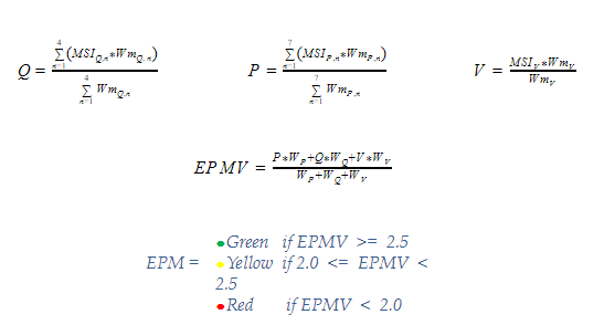
In the cases where a Product is not currently collecting a required measure/metric, the MSI of that metric is assigned a value of 0 (Grey).

4.6 Evaluating the EPM – Dashboard Creation

With the EPM calculated, dashboards are created that capture EPMs for all products and provide a snapshot of product maturity. With the appropriate algorithms, trend arrows are added to show tendencies and provide a signal that assists in the investigation and/or action that may be necessary to correct adverse conditions. Levels of detail are also provided allowing ‘drill down’ to get to the individual areas of interest.

Figure 3 illustrates a high level dashboard providing overall summary of products. Figure 4 shows the breakout organized by Threads. Figure 5 provides an example of a lower level detailed view into one of the products. Note that MSIs on dashboards in dark grey (or black) indicate there was no data collected.  In addition, the trend arrow is not displayed.  Additional dashboards include the ‘extended’ metrics (see Figure 6).

Figure 3 – Product Summary Dashboard

Figure 4 – Thread Summary Dashboard

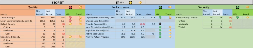
Figure 5 – Product Detailed Dashboard

Figure 6 – Thread Summary with Extended Metric Dashboard

4.6.1 Trend Icons

Trend arrows (which indicate tendencies for a given metric to move in a particular direction) are assigned to each metric based upon a calculation of simple difference or by some other more precise method. Application to the fundamental (and extended) metrics uses a statistical approach. Application to the changes in EPM or MSI uses a simplistic approach based solely on the previous value.

4.6.1.1 Metric Trends

Although the difference method is easy to determine (subtract the current value from the previous), it will tend to be a bit over-responsive to sudden changes in the value of the metric. Because it only looks at the last two data points, noisy data can mask the true signal. 

The method used (calculation of change over monotonically increasing or decreasing values) involves using the most recent history of the metric’s value to help smooth out the tendency of noise to drive oscillations in any potential trend.

A running average of metric values is calculated over the whole period of available data. Regions are then determined where the change in direction (increasing/decreasing value) occurs. The last region (most recent data) is evaluated to determine the degree of change in the average (via a calculation of linear slope) and a determination of trend is then calculated based on the value of that slope. 

Even though this process for calculating the trend accounts for noisy and oscillating data fairly well, severe swings in data may still cause trend arrows to flip in orientation. One should consider evaluating trends based on two consecutive trend values in the same direction. 

4.6.1.2 EPM and MSI Trends

Both the EPM and MSI trend values are computed based on the weighted average of their component parts. The MSI value from the individual metric trends; the EPM value from the average of the three metric group trend values.

4.7 Extended Metrics

Although the fundamental metrics are required of all products, additional measures can (and should) be monitored and evaluated if they are good indicators of a product’s set of performance goals. These ‘extended’ metrics are developed and used in much the same way as the base metrics: they have an operational definition, thresholds are assigned for each and evaluations are made against specific goals that each metric (or set of metrics) was designed to measure.

Since these extended metrics are specific to each individual product (although many are somewhat common) they are not used in the evaluation of the product’s EPM.

Examples of extended metrics are provided in Table 19 with a sample chart (and thresholds) in Table 20.

Table 19 – Sample Extended Metrics

Table 20 – Example Chart – System Availability

By: Mike Mangieri
Senior Principal Process Engineer
Business Transformation Institute, Inc.